The Covid-19 Lab Leak Theory Is a Textbook Example of Confounding
Ever since the start of the Covid-19 pandemic, there has been widespread speculation on the origins of the virus. The ’lab leak’ theory states that Covid-19 was created in the Wuhan Institute of Virology and had accidentally espaced. A number of recent studies (Holmes et al. (2021), Worobey et al. (2022)) have provided strong evidence against it.
From a statistical point of view, the lab leak theory is the result of confounding. Ignoring the causal relations allows for simplistic explanations that on a second look do not hold water. This post will provide a few simulated examples on how this confounding arises.
Modeling the causes of outbreak as a causal DAG
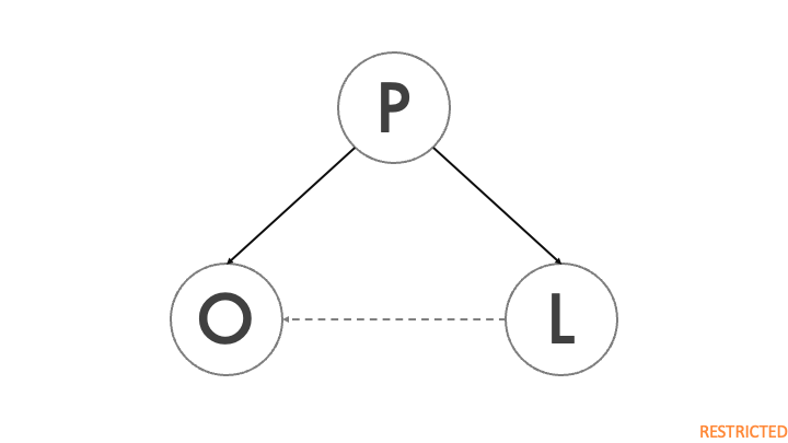
The figure shows a simplified DAG of a Covid-19 outbreak. P denotes the city population, L indicates the presence of a major virology lab in the city, and O is the outbreak of a previously unidentified virus. The city population directly impacts the presence of a lab, because large scientific institutions are more likely to be present in larger cities. On the other hand, population also has an impact on the probability of a major disease outbreak, as a highly contagious disease will be able to spread to more people in a shorter amount of time. The dashed arrow represents the impact of the lab on the outbreak, which is the lab leak theory. As Holmes et al. (2021) point out, a lab leak has only happened once, so this effect is likely to be extremely weak.
Population is a confounder, because it affects both the outbreak and the presence of a lab. Without conditioning on P, the backdoor is not closed and any attempt to relate the outbreak to the presence of a lab will be highly misleading.
Creating a simulation based on the DAG
First, we’d like to create a synthetic dataset of cities and check whether an outbreak has taken place and whether there is a lab in the city. Both depend on city population.
We model city population with a gamma distribution to mimic the skewness observed in the real world with respect to city size. Most cities are small and only a few are very large metropolitan areas. The unit for the population is millions of inhabitants. For this example, we will set the number of cities to one million so that any statistical artifact will be clearly observed. This is only for illustrative purposes and might lead to our simulated world having a larger population than the Earth. Here’s how to do it in R:
N <- 1e6
population <- rgamma(N, 2, 0.4)
Let’s check the population quantiles:
0%     25%    50%    75%    100%
0.004  2.405  4.198  6.728  42.103
Our smallest city has a population of 4000, and the largest of 4 million, which is a realistic range.
Both the presence of a lab and the disease outbreak will be modeled as Bernoulli random variables. As a Bernoulli distribution is parametrized by a probability, we will use the sigmoid function to relate the population to the respective variable and keep the possible values between 0 and 1:
sigmoid <- function(x) 1 / (1 + exp(-x))
The probability of a lab being in a city is given by:
prob_lab <- sigmoid(-3 + 0.2 * population)
A coefficient of 0.2 is telling us that for every additional million citizens, the odds of housing a lab in the city increase by a factor of exp(0.2) = 1.22. The intercept of -3 helps us set a realistic range (i.e., what would happend if population is equal to zero?). Again, let’s check the resulting probabilities:
   0%   25%   50%   75%  100%
0.047 0.075 0.103 0.161 0.996
The probability of the smallest city of having a large lab is very low, around 4%, while for the largest city with a population of over 40 million it is almost 100%.
Using this probaiblity, we generate the lab variable:
lab <- rbinom(N, 1, prob_lab)
We repeat the same procedure for disease outbreak:
prob_outbreak <- sigmoid(-7.5 + 0.15 * population + 1e-4 * lab)
Here, we are also including a very small effect (1e-4) for the presence of a lab, because leakages have happened, but only once.
This corresponds to the dashed arrow in our DAG.
The resulting probabilities are as follows:
   0%   25%   50%   75%  100%
0.001 0.001 0.001 0.002 0.234
A major outbreak is highly unlikely in smaller cities, but becomes more likely as the city becomes bigger.
Finally, we also simulate the outbreak variable and put all variables in a data frame:
outbreak <- rbinom(N, 1, prob_outbreak)
df <- data.frame(population = population, lab = lab, outbreak = outbreak)
The lab is leaking like a sieve!
Time to fit some models!
We will be using the brms package to fit Bayesian logistic regressions. First, we fit the confounded model, which means ignoring the population and focusing only on the presence of the lab.
By default the bernoulli family uses a logit link (i.e. sigmoid).
confounded_reg <- brms::brm(formula = outbreak ~ lab,
                            data = df,
                            cores = 4,
                            family = brms::bernoulli(),
                            backend = "cmdstanr")
After checking that we do not have any computational issues, we check the model summary:
Population-Level Effects:
          Estimate Est.Error l-95% CI u-95% CI Rhat Bulk_ESS Tail_ESS
Intercept    -7.08      0.04    -7.16    -7.01 1.00     3086     2276
lab           0.54      0.09     0.36     0.71 1.00     3104     2298
According to this model, the presence of a virology lab increases the outbreak odds by a factor of exp(0.54) = 1.71.
Looking at the credible interval for lab, realistic values for the odds ratios are between exp(0.36) = 1.43 and exp(0.71) = 2.03.
This means that the mere existence of a lab would almost double the odds of a disease outbreak in the worst case.
Before we grab our pitchforks and burn down the lab, we remember that confounding can be a problem when estimating a model. Fortunately, we also have information on the city population, which we can easily plug into our logistic regression.
causal_reg <- brms::brm(formula = outbreak ~ lab + population,
                            data = df,
                            cores = 4,
                            family = brms::bernoulli(),
                            backend = "cmdstanr")
Again, CmdStanR should give you a warning in case there are any computational issues like divergences.
As there are no problems, we check the model summary:
Population-Level Effects:
           Estimate Est.Error l-95% CI u-95% CI Rhat Bulk_ESS Tail_ESS
Intercept     -7.92      0.06    -8.03    -7.80 1.00     2571     2381
lab            0.02      0.10    -0.17     0.20 1.00     2631     2659
population     0.15      0.01     0.13     0.16 1.00     2930     2670
Including population into the model changes the results completely!
The lab variable is now zero on average and the credible interval reinforces the notion that the effects is neither negative nor positive.
Only population has a clear positive effect on the outbreak, with an approximate increase of the odds ratio by a factor of exp(0.15) = 1.16.
Note also that the estimated error for the population variable is much lower than the error we had for the lab variable in the first model.
In summary, just by conditioning on the confounder population we were able to close the backdoor that made it look like the presence of a lab has a very large impact on the probability of an outbreak.
Two slightly different models that lead to very different conclusions!
Some limitations
Of course, this example is far from perfect. For starters, it is just a simulation and reality is much messier than what our toy data set might suggest. Moreover, there are hidden assumptions in the data that might not be obvious at first. Cities are only distinguished by population and lab presence, which means that everything else is assumed to be equal.
For example, the Covid-19 outbreak was likely caused by species like racoons or civets, which are known to be carriers of viruses that can spread to humans and are sold at wet markets. Therefore, we assume implicitly that every city in our data set has exactly one place similar to the wet market in Wuhan, regardless of its population size. This is a highly unplausible assumption.
Conclusion
In this simple example, we simulated the results from recent studies on the origins of Covid. We showed that confounding can lead to the wrong conclusions and that it is always worthwhile to think about the causal relations between variables. Spurious correlations are everywhere and if they reinforce our existing opinions, it is tempting to think they are true. The lab leak theory might be yet another example of us forgetting that ‘correlation is not causation’.
References
Holmes, E. C., Goldstein, S. A., Rasmussen, A. L., Robertson, D. L., Crits-Christoph, A., Wertheim, J. O., … & Rambaut, A. (2021). The origins of SARS-CoV-2: A critical review. Cell, 184(19), 4848-4856.
Worobey, M., Levy, J. I., Malpica Serrano, L., Crits-Christoph, A., Pekar, J. E., Goldstein, S. A., … & Andersen, K. G. (2022). The Huanan Seafood Wholesale Market in Wuhan was the early epicenter of the COVID-19 pandemic. Science, 377(6609), 951-959.
Follow me on Twitter!