The Problem With Interpreting Biased Coefficients
One of the first things people learn about regression analysis is how to interpret coefficients and it is seemingly easy. But coefficient interpretation can also lead to some subtle pitfalls. Suppose a regression is given by \(y = \beta_0 + \beta_1 x_1 + \beta_2 x_2 + \varepsilon\). If we increase \(x_1\) by one unit and at the same time keep \(x_2\) constant (the so called ceteris paribus assumption), then \(y\) would change by the amount \(\beta_1\). In other words, \(\beta_1\) is the effect of \(x_1\) after controlling for \(x_2\). However, there are some problems with this approach. First, we assume that there is a ’true’ parameter that we try to estimate and an estimate can be biased. While the model might create the illusion that it is taking care of the problematic bits, it might actually make matters worse. Second, it is not clear what kind of effect we are are trying to approximate with our estimate. Effect is a very general and unprecise word. In the end, it all depends on what the model is supposed to deliver: a good prediction or an explanation of relations between variables. In this post, I’ll do the following
- Revisit the statistical mantra correlation is not causation
- Introduce a classical example of biased coefficients from the econometric literature
- Explain why going to a checklist of coefficient biases does not guarantee that the coefficients really are what they seem
- List types of biases which can lead to unexpected behavior
There will also be some short simulations in R to illustrate the problems.
Correlation is not causation
Correlation is not causation has become a mantra of statistics – a mantra that is constantly thrown out of the window in subtle ways. After running the regression, we get the estimates \(\hat \beta_0, \hat \beta_1\) and \( \hat \beta_2\) for the coefficients. Strictly speaking, the coefficients only capture the correlation between \(y\) and the regressors. To be more exact, the partial correlation, i.e. the correlation after controlling for the other regressor. However, if there is no confounding, the effect of the coefficients can be interpreted causally. This post does not discuss these conditions, but they are well explained in Statistical Rethinking by Richard McElreath or the Book of Why by Judea Pearl.
By making this distinction between correlation and causation, we automatically introduce a distinction in the application of a regression. If the model fulfills the conditions for causal interpretation, then the coefficients quantify the causal effect of the regressors. On the other hand, if we remain in the realm of correlation, the coefficients are measures how well a regressor can predict a dependent variable through their partial correlation. For example, chocolate consumption is a good predictor of income per capita, but it’s not it’s cause – although some of us wish eating chocolate would make you richer.
When making predictions, we are interested in how good our prediction is and if any given variable in the regression is actually contributing to improve the prediction. Variables that do not have a good predictive power should be removed from the regression, as they will unnecessarily introduce more variance to the predictions. This can be done with the help of cross-validation, as well as information criteria such as the AIC or the BIC. However, as long as the prediction is good, it is not so important if the coefficients are biased. In fact, models with biased coefficients can outperform causal models.
Example: education and income
Let’s take a classical example from econometric literature – quantifying the effect of education on income. The government is interested in how much an extra year of education (financed by taxpayer’s money) contributes to having a better income in the future. However, there is a potential confounder: intelligence. More intelligent people are likely to earn more due to their intelligence. At the same time, more intelligent people are likely to get more years of education. The problem here is that while it might be easy to get information on income and education through a survey, gathering information about intelligence might be more difficult (when was the last time a pollster asked you about your IQ?). The confounding is shown in the following graph: education (ED) has a direct effect on income ($), while intelligence (IQ) has a direct effect on both education and income
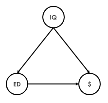
Income ($), education (ED) and IQ
The true relation between variables is \(income = \beta_0 + \beta_1 \cdot education + \beta_2 \cdot intelligence + \varepsilon\). By leaving, \(intelligence\) out the estimate \(\hat\beta_1\) will be biased. But, does it matter? Well, if the aim is to spend taxpayers’ money in the most effective way, you definitely want do close the backdoor path and get the causal effect. What if spending of education has no effect on income after all? With a biased model, it is not possible to tell. If you are just trying to predict income, then the only thing that really matters is whether the prediction is good. This can be measured for example by the root mean squared error applied to a left-out part of the data. The coefficient will tell you that the correlation between education and income is positive. And with inference that it is different from zero. However, the effect only measures correlation not controlling for intelligence, so there is no way to interpret the coefficient beyond its predictive power.
Why worry about biased coefficients?
The application of the problem should dictate whether biased coefficients need to be dealt with. For prediction, biased coefficients should not matter that much. What matters is that the prediction is good, which usually means minimizing variance and bias as much as possible. Coefficient interpretation is just an afterthought. For causality, the story is different, because you need to be very careful to avoid confounding. Things to avoid are post-treatment bias, omitted variable bias, conditioning on a collider, or reverse causality. Without an extra construct such as a DAG that captures the relations between the variables, it is impossible to deconfound the model using only regression.
Those two cases are quite clear-cut. However, there is a third case which I find problematic. It is “best-practice” for researchers to go great lengths to avoid certain kinds of bias, like omitted variable bias. This generally acknowledges the presence of confounding factors that can distort coefficient estimates. At the same time, there is no well-defined strategy to actually understand the nature of confounding. Some variables might be added or removed without a clear plan causing the coefficients and their significances to vary wildly. Focusing on the bias and not on the confounding structure of the variables is short-sighted – it is like treating the symptoms while ignoring the illness. And it creates a false illusion that you are dealing with the bad aspects of the model, while there might still be plenty of pitfalls. Correlation suddenly starts to look and feel deceivingly similar to causation.
Still, there are types of non-causal biases which are problematic in most cases and I will discuss some of them in the next section.
Non-causal biases
There are of course three cases which come to mind where bias might be undesirable or misleading: multicollinearity, measurement error and spurious correlations.
1. Multicollinearity
Multicollinearity is the inclusion of superfluous information into the model. Back in the regression example with two variables, we had \(y = \beta_0 + \beta_1x_1 + \beta_2x_2 + \varepsilon\). In the extreme case of perfect multicollinearity we have \(x_1 = x_2\). By simple algebra, we can rewrite the regression as \(y = \beta_0 + (\beta_1 + \beta_2)x_1 + \varepsilon\). The problem: there are infinite combinations of \(\beta_1 + \beta_2\) that would have the same coefficient as a result. Therefore, the effects and signs of \(\beta_1\) and \(\beta_2\) will be arbitrary and misleading. Besides, the variance of the estimated coefficients \(\hat \beta_1, \hat \beta_2\) will be extremely large and the estimation method of the regression is likely to break, even if the multicollinearity is not perfect. In R you could write:
N <-  1000
x_1 <- rnorm(N, mean = 0, sd = 2)
x_2 <- x_1 + rnorm(N, mean = 0, sd = 0.001) # x with a small amount of noise
y <- 2 - x_1 + rnorm(N, mean = 0, sd = 1) # True effect of x_1 is -1

fit_multi <- lm(y ~ x_1 + x_2)
summary(fit_multi)
Which results in
Coefficients:
            Estimate Std. Error t value Pr(>|t|)
(Intercept)   1.9451     0.0325   59.90   <2e-16 ***
x_1         -25.0170    32.6523   -0.77     0.44
x_2          24.0044    32.6532    0.74     0.46

Residual standard error: 1.03 on 997 degrees of freedom
Multiple R-squared:  0.794,	Adjusted R-squared:  0.793
F-statistic: 1.92e+03 on 2 and 997 DF,  p-value: <2e-16
By looking at the \(R^2\) the model can explain around 80% of the variation in \(y\), but the regressors are insignificant. The standard errors are very large. However, the coefficients of the \(x_1\) and \(x_2\) add up to approximately \(-1\), which is the true coefficient. The F-statistic also indicates that although both coefficients are not significant separately, they are jointly different from 0. If you run the code a couple of times, you will notice that the coefficients jump around quite a bit, but the coefficients always add up to almost \(-1\).
2. Measurement error
Let’s go back to a simpler model with one variable: \(y = \beta_0 + \beta_1 x + \varepsilon\). Suppose we are only able to measure variable \(x\) with a certain error \(\eta\) with zero mean and unit variance. The regression then becomes \(y = \beta_0 + \beta_1(x + \eta) + \varepsilon\). As \(\hat \beta_1 = \displaystyle \frac{Cov(x, y)}{Var(x)}\), the variance of \(x\) would increase, if we measure it with an error. If \(x\) and \(\eta\) are uncorrelated, then \(Var(x + \eta) = Var(x) + Var(\eta) > Var(x)\). Thus, the estimated \(\hat \beta_1\) will tend to be lower than it should be, as the denominator is larger. This is called attenuation bias. This is a bias that is not causal, as it does not depend on the relation to other variables. A short simulation of this scenario:
N <-  1000
x <- rnorm(N, mean = 2, sd = 2)
y <- 3 + 10 * x + rnorm(N, mean = 0, sd = 1)

noisy_x <- x + rnorm(N, mean = 0 , sd = 1)
fit_attenuated <- lm(y ~ noisy_x)
summary(fit_attenuated)
The regression summary shows
Coefficients:
            Estimate Std. Error t value Pr(>|t|)
(Intercept)    7.257      0.361    20.1   <2e-16 ***
noisy_x        7.970      0.120    66.5   <2e-16 ***
---
Signif. codes:  0 ‘***’ 0.001 ‘**’ 0.01 ‘*’ 0.05 ‘.’ 0.1 ‘ ’ 1

Residual standard error: 8.44 on 998 degrees of freedom
Multiple R-squared:  0.816,	Adjusted R-squared:  0.815
F-statistic: 4.42e+03 on 1 and 998 DF,  p-value: <2e-16
In this case, the coefficient estimate is around 8, which is 20% lower than the true coefficient from the simulation. This bias cannot be removed by deconfounding the model. The noisier regressor is also more likely to produce worse predictions.
3. Spurious correlations
The third type of bias is when spurious correlations are introduced. One example comes from time series, when trying to regress a random walk on another random walk. Another simple example can be shown through collider bias. Suppose we want to find out whether we can predict food quality in restaurants given their location and revenue (this example for collider bias is taken from Statistical Rethinking). The true relation between variables is given by the following graph, where $ is revenue, F is food quality and L the location:
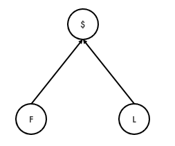
Revenue ($), location (L) and food quality (F)
Note that food quality and location are completely independent. Let’s now write some code to simulate the graph:
N <-  1000
food <- rnorm(N, 0, 1)
location <- rnorm(N, 0, 1)
revenue <- 1 + 10 * food + 5 * location + rnorm(N, 0, 1)
If we run a simple regression with only revenue as an explanatory variable, we will a measure of the correlation between revenue and food quality. This effect can never be causal, as food quality causes higher revenue and not the other way around. Therefore, in this example there is no way to deconfound the model. We get the following result:
lm(formula = food ~ revenue)

Coefficients:
            Estimate Std. Error t value Pr(>|t|)
(Intercept)  0.13194    0.02592    5.09  4.3e-07 ***
revenue      0.08844    0.00101   87.65  < 2e-16 ***
---
Signif. codes:  0 ‘***’ 0.001 ‘**’ 0.01 ‘*’ 0.05 ‘.’ 0.1 ‘ ’ 1

Residual standard error: 0.474 on 998 degrees of freedom
Multiple R-squared:  0.885,	Adjusted R-squared:  0.885
F-statistic: 7.68e+03 on 1 and 998 DF,  p-value: <2e-16
If we include location in the regression, something strange happens. By conditioning on the collider, information flows from food quality to location. Suddenly, location is a significant predictor of revenue. However, remember that both variables are independent. The results from the regression can be summarized as follows:
lm(formula = food ~ revenue + location)

Coefficients:
             Estimate Std. Error t value Pr(>|t|)
(Intercept) -0.093918   0.005796   -16.2   <2e-16 ***
revenue      0.099517   0.000231   431.7   <2e-16 ***
location    -0.495256   0.003455  -143.3   <2e-16 ***
---
Signif. codes:  0 ‘***’ 0.001 ‘**’ 0.01 ‘*’ 0.05 ‘.’ 0.1 ‘ ’ 1

Residual standard error: 0.102 on 997 degrees of freedom
Multiple R-squared:  0.995,	Adjusted R-squared:  0.995
F-statistic: 9.32e+04 on 2 and 997 DF,  p-value: <2e-16
The collider bias has such a large impact on the coefficient’s location that is seems to have a significant effect, when in reality is has no effect at all. It is even larger than the effect of revenue on food quality. This is a spurious correlation. This one is very hard to catch with traditional statistical techniques: the revenue coefficient only changes slightly, the AIC and BIC prefer the confounded model, and the common regression plots (in R calling plot on an lm object) will not reveal any suspicious patterns. However, it is important to keep in mind that while this bias might lead to a wrong idea of the relations between variables, it might still lead to better predictions.
Summary
While coefficient interpretation is a key component of regression analysis, there are many pitfalls related to confounding and biases. In any project that uses statistics, the application should determine whether you should worry about confounding or not. It is especially dangerous to pretend to be dealing with biased coefficients, when in reality the confounding might still not have disappeared. Depending on the situation, the interpretation could just be invalid. Prediction and causality questions should be separated from one another as much as possible. However, there are some types of bias that are usually undesirable or misleading. Some examples are multicollinearity, measurement error and spurious correlations.
Using statistical or machine learning models in a mechanical way rarely is a good strategy for data analysis or prediction models: it is crucial to define the project scope and to understand the subtleties of the methods. Yes, it is necessary to deal with coefficient biases. However, the how might change depending on the application.