Assumptions Matter: Ignoring Them Can Invalidate Your Findings
Earlier this week, I attended an amazing talk at PyConDE / PyData 2023 on data engineering. At some point, the speaker made the point that data engineers have to understand basic statistics for their jobs and showed a list of common statistical tests that people should know. Then, he made a lengthy real-world example using a t-test. I am all for it when it comes down to statistical literacy, and believe that a little understanding about probabilities would help a lot of people make more informed judgements.
However, there were two things I found a bit troubling about this message. First, some people might think that statistics is only a set of tests that can be imported from scipy, and that can give you infallible insights about your data – after all, the test is making the decision so that you don’t have to make it, right? Second, the hard thing about statistics is not necessarily understanding the toolbox, but reminding yourself that everything depends on the theoretical assumptions of each method.
This blog post will make the following points: 1) statistical tests can and should be reformulated as models most of the time, 2) knowing the assumptions is key to understand the reliability of your model. We’ll also do a short simulation example in NumPy to illustrate how to break a test and how you can fix it with standard tools.
Statistical tests are a poor substitute for models
Statistics is much more than a canonical list of tests. Statistical tests come from a time in which many of the computations had to be done by hand. In reality, many well-known tests are just probabilistic models in disguise. Jonas Lindeløv has an amazing list of tests reformulated as a model. The main issue is that it is tricky to compute a regression manually. Want to estimate a linear regression? Well, to estimate the regression parameters you have to multiply a bunch of matrices with each other. Not so fun. Oh yeah, and don’t forget that matrix inversion. Even less fun. Want to estimate a t-test? Calculate the mean and standard deviation and you’re pretty much good to go! What’s not to like, huh?
Luckily, we have computers nowadays. They abstract away a lot of the tedious work that makes university students hate statistics in the first place (yes, computing standard deviations by hand is extremely boring). There’s no reason to use a test if you can use a model that gives you flexibility with regards to the type of information you can include. You can even use a Bayesian model that allows for even more flexibility regarding the assumptions you include into the model, and go crazy with the likelihood or add a hierarchical structure to your model.
If you don’t know the assumptions, you don’t understand the method
This leads me to my second point: assumptions. Every statistical test relies on assumptions. Usually, the assumption is related to the Central Limit Theorem (CLT), which provides a powerful result that under certain cirumstances the mean of a random variable is a Gaussian, no matter what the distribution of that random variable is. It is one of those results that seem like mathematical magic. (If it’s the first time you hear about the CLT, consider spending time understanding its meaning and implications.) Unfortunately, the assumptions that underlie the CLT are often not fulfilled.
Do you have to be a math genius to understand the assumptions? I don’t think so, but it might take some work. Let’s check the Wikipedia article for the t-test. One of the key assumptions is that the sample mean $\bar X$ of the data needs to be normally distributed. How do I know that? The CLT gives you the answer to that: the mean of a (sufficiently large) sample is normally distributed when the single observations are independent from each other (this is the more general version of Lyapunov that does not assume identical distribution of the observations as long as the variance of any individual observation doesn’t get out of whack). Informally, independence means that there is no information shared between observations. This implies that two independent variable cannot be correlated. As we will see, this is quite a restrictive condition.
Tests break down easier than you expect
Breaking a test is easier than you might think. In the real world, true independence is quite rare. Even small amounts of correlation between observations can invalidate a test that relies on the CLT. This might happen in a very subtle way when you have a grouped structure in the data like data from multiple countries, or multiple measurements for the same individual.
To illustrate this, let’s do a small simulation study. We will use the following libraries:
from scipy.stats import ttest_1samp
from scipy.linalg import block_diag
import numpy as np
import statsmodels.api as sm
import seaborn as sns
We will simulate a population with 10 different groups (n_groups) with 100 observations in each group (group_size)
group_size = 100
n_groups = 10
group = np.repeat(np.arange(0, 10), repeats=group_size)
total_size = group_size * n_groups
reps = 100
group is a variable that contains the group assignment for each observation and reps determines the number of synthetic populations that we will create.
To ensure reproducibility we set the seed and pass it to a random number generator:
seed = 100
rng = np.random.default_rng(seed)
We define a baseline that consists of perfectly independent observations:
independent = rng.normal(size=(total_size, reps))
Next, we generate a data set with a clustered structure. For this, we use a block diagonal matrix, which makes sure that correlation between groups is zero, while within-group correlation is uniformly sampled between 0.1% and 5%. Keep in mind that a correlation of 5% is usually considered to be extremely low, and you might be tempted to think that it will not have a big impact on the results.
We use np.fill_diagonal to make sure that all observations have unit variance:
covariance = block_diag(
    *[rng.uniform(0.001, 0.05, (group_size, group_size)) for _ in range(n_groups)]
)
np.fill_diagonal(covariance, 1)
Finally, we use the block diagonal covariance matrix to generate 100 synthetic populations of size 1000 with a multivariate normal distribution. All the distribution means are set to 0:
clusters = rng.multivariate_normal(
    mean=np.zeros(total_size), cov=covariance, size=reps
).T
Great! Now that we have our two synthetic populations we can see what happens with a simple one-sample t-test that checks whether the population mean is equal to zero. Assuming a significance level of 5%, you’d expect to see a type I error around 5% of the time. This means that we would falsely reject the null hypothesis (here: the sample mean is equal to zero) around 5% of the time. Luckily, we already have 100 repetitions of our population. If we do a test for each repetition, we’d expect that the p-value will be below 0.05 around 5 times. We also know for sure that the true mean is zero, so rejecting the null hypothesis more than 5% of the time should be a red flag.
(ttest_1samp(independent, popmean=0).pvalue < 0.05).sum()
>>> 5
In this case, we would wrongfully reject the hypothesis “sample mean == 0” around five times, which matches exactly what you’d expect from the theory. What about our clustered example?
(ttest_1samp(clusters, popmean=0).pvalue < 0.05).sum()
>>> 34
Ouch! We are off by a lot. This shows very clearly how a very small amount of correlation within groups can completely invalidate a statistical tests, even though by design our data has zero mean.
Why does this happen? The CLT assumes independence for the sample mean to be approximately a Gaussian distribution. If this assumption is not met, then pretty much anything can happen. Let’s compare the densities of the standardized means for each scenario:
sns.kdeplot(clusters.mean(axis=0) / clusters.std(axis=0))
sns.kdeplot(independent.mean(axis=0) / independent.std(axis=0))
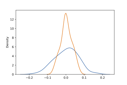 In short, the distribution of the standardized mean is much wider for the clustered scenario (blue line) than what is required by the CLT (orange line). A wider distribution in this context translates directly into more test rejections.
Fixing the test with a linear regression
We already mentioned that most tests can be defined as a model. This gives us a few more tools to deal with correlation between observations, especially when we know that there might be a clustered structure in the data.
We will estimate the t-test as a regression, and we will use a clustered covariance matrix in the model to correct the standard errors and get valid p-values. The fit method of the OLS regression in the package statsmodels accepts a cov_type argument that can be used to define a clustered covariance matrix. Moreover, you have to pass the grouping variable as a keyword with cov_kwds.
To do the t-test, as a regression we pass the variable of interest as a (y) and an array of ones as an (X).
Fitting the regression for all the clusters, looks like this:
pvalues = []
for cluster in clusters.T:
    value = (
        sm.OLS(cluster, np.ones(total_size))
        .fit(cov_type="cluster", cov_kwds={"groups": group})
        .pvalues
    )
    pvalues.append(value)
pvalues = np.concatenate(pvalues)
We are using the p-values from the t-test on the intercept that is done by default in statmodels to check whether our population mean is equal to zero:
(pvalues < 0.05).sum()
>>> 8
This is not exactly 5, but it is in the same ballpark as the theoretical ideal. It might be a bit higher due to randomness. Most importantly, it is not as far off as with the vanilla t-test, so in this case the results would be more trustworthy.
Key takeaways
I hope that this short example showed that it is never a good idea to use statistical methods without understanding the assumptions. Unfortunately, there is no list of the top ten statistical procedures that everyone should know. Real-world data is complicated and the context of the data determines the method. Moreover, statistics and probability are the language of uncertainty, and it’s not the most intuitive language to learn. There are no shortcuts.
The next time you use a statistical test ask yourself the following questions:
- Do I understand the assumptions behind this method? Do I need to run a simple simulation to uncover potential pitfalls?
- Am I integrating all the information available?
- Is there a way to turn this test into a model, and are there additional tools in a model that could be used?
To sum up, taking the time to thoroughly understand the assumptions and context of statistical methods is crucial for producing trustworthy and accurate results. I hope that this blog post provided some insights into why this is important and how to do some quick checks in practice with Python.
GitHub: @flaviomorelli Mastodon: @flaviomorelli@sigmoid.social Twitter: @mexiamorelli